Energy in a Mark II Economy

Important Note. If you have read this paper previously, always look in What’s New first; and, if an experiment has been added since your last reading, look there next. Unfortunately, the changes made today will necessitate a complete re-reading. Normally, you will find everything you need to read here and in any experiments you have not yet seen. I hope you have taken my advice about downloading new copies of this paper and the spreadsheets whenever you work on this project. This is an intentionally open-ended paper that takes advantage of web publication to do something that cannot be done in the print literature – except that many academics write paper after paper that are no more than progress reports on work done previously and contain no new ideas. Thus, on the tree of “publish or perish” no wholesome fruit grows.

This is the beginning of a complete revision of this paper to exploit a new relation between emergy and the ratio of Energy Returned to Energy Invested (ER/EI) and to introduce a new routine for computing two of the three values for ER/EI. Also, the original spreadsheet will be retired in favor of http://www.dematerialism.net/Mark-II-Economy-New.xls, which will be renamed http://www.dematerialism.net/Mark-II-Economy.xls, the name of the old spreadsheet. Convergence will be about 100 times faster; however, many sections of this paper will have to be altered and, hopefully, simplified to account for the differences in the two spreadsheets. The spreadsheet for constant sector populations is http://www.dematerialism.net/Mark-II-Economy-CSP.xls.

It has come to my attention that some people do not see the point of building an economy that models the American and other hypothetical economies in an idealized way that is guaranteed to be less wasteful than every real economy of the same type. Unfortunately, some things that there is no need to say should be said anyway.

The Base Case (BC) is a steady-state idealization of an American-style market economy that is guaranteed to be less wasteful than the real economy because the differences between the upper classes and the working classes are less extreme, there is no financial or monetary system with banks and stock exchanges and so on, and there is no government and military sector. However, even the idealization of an American-style market economy is certain to be more wasteful than any real economy in which every single person receives exactly the same share of the national economic dividend regardless of what he does or doesn’t do. Although there is the cost of buying and selling and there is a middleman from the commercial sector interposed between consumers and the sectors and between sectors, no one can become richer by means of the market. Therefore, the savings indicated for a move from BC to the No-Managers Case (NM) are certain to occur in real life and they will probably exceed the savings indicated by the model.

The situation is the same for moves from NM to the No-Commerce Case (NC) and from NC to the No-Commerce-No-Managers Case (NCNM). Let us characterize the worst-case scenario for each case with an asterisk and the best-case idealization with an unembellished symbol since the cases in the model are the best-case idealizations. Then, the order of energy consumption from greater to less for identical standards of living for workers whether on active duty or furloughed is as follows: E_BC* > E_BC > E_NM* > E_NM > E_NC* > E_NC > E_NCNM*> E_NCNM or, more likely, E_NCNM* = E_NCNM. Since the reader is aware of the vital nature of our need to reduce our energy budget in the wake of Peak Oil, the purpose of the exercise should now be abundantly clear, however see the list of four educational goals in To the Reader below.

Speaking of things that I have had “no need to say”, when I say No Managers, I do not mean that no one will manage. I mean that managers will be paid the same as other workers; and, since the worker is the manager’s client, the workers ought to select their managers from among themselves. The comic strip Dilbert reminds me that managers who are not competent workers are generally incompetent managers as well.

Since the macros are re-written frequently, it would not be a bad idea to learn their names so that you can click on the Tools Menu, click on Macros, click on Macros on the macro list, and find what keys to press for each macro. See the tables of macro names and what each one does in the new Appendix A. In the meantime, follow my instructions in the experiments but look up each macro in Excel’s drop down menu before you use it. Before long, you should become familiar with my style in naming macros with Incr standing for increment, NR standing for Newton-Raphson, Iter standing for iteration, etc.

I have changed the spreadsheets parameters so frequently that most of the tables that had been filled in during earlier experiments no longer have the correct values. This is fine as I expect the reader to repeat the experiments on his copy of the spreadsheet and fill out the tables correctly.

Lately, I have been working on a new spreadsheet at http://www.dematerialism.net/Mark-II-Economy-New.xls (renamed http://www.dematerialism.net/Mark-II-Economy.xls for this revision) on which the fractions retained for salaries is the same for every sector; therefore, only the commercial equation is used to find the one fraction, and the other equations that balance salaries with expenses can be used to compute the fraction of the population attached to that sector. The fraction of the population supported by commerce makes the sum of the fractions equal to 1.0. In the Base Case, I have found the set of δ_ij and η_i that match the cash fractions spent by consumers on the four commodities and the energy fractions consumed by the four sectors tabulated by the DOE for the United States on or about the year 2000. Thus, http://www.dematerialism.net/Mark-II-Economy.xls will return somewhat different results than were reported in this paper previously. This is reported in Experiment 16. Further, in Experiment 17, I have chosen δ_EE so that ER/EI^o (now defined correctly) matches the average ER/EI^o of the slate of fossil fuels used in the United States. Also, I have chosen the factor by which the consumption of residential units and manufacturing units for managers exceeds that of workers to match the income distribution in the United States between the upper 10% and the lower 90%.

To the Reader

The Mark II Economy provides a computational laboratory in which the energy analyst can perform experiments on a simplified economy that replicates many of the important features of a real economy. The Mark II Economy is simple but not very simple. The governing equations are troublesome enough that mathematical analysis might be replaced by numerical experiments in most instances. Also, numerical simulation is a useful tool to verify conclusions reached analytically. When you download the spreadsheet, be sure to Enable Macros. They are needed to follow this discussion, and they are safe. If you are unable to do this, lower the security level under Security under Macros on the Tools menu in MS Excel. Also, if the window that says “This workbook contains links to other data sources” pops up, click on Don’t Update.

The Mark-II-Economy achieves four important goals:

1. To show how energy is related to money. One may estimate the increase in the total energy budget (E) associated with a diversified monetary investment by multiplying the capital, operating, and other costs of the investment by the E/GDP ratio. See Experiment 1.

2. To eliminate the confusion regarding the ratio of energy returned to energy invested (ER/EI). Three separate ER/EI ratios are defined depending upon what is included in the energy invested term. The quantity EI^o includes only the direct energy costs of providing the net energy to the economy; EI (with no superscript) includes the indirect expenses but not those incurred by commerce; EI* includes, in addition, the energy costs of commerce. ER/EI^o and ER/EI are independent of political economy as the standard of living of the workers remains constant when the political economy changes.

3. To illustrate graphically the effect of lowering the ER/EI* ratio due to substituting a less efficient technology for the technology that preceded it chronologically. One sees the total energy budget, E, approaching infinity as ER/EI* approaches 1.0. (Chart 2) In this paper, I have defined Energy Returned to be the total energy extracted or produced. This is the sum of the energy delivered and the energy invested. An alternative definition counts only the energy delivered. This has the advantage that it is easily computed in practice. If the alternative definition is used, each of ER/EI ratios is reduced by exactly 1.0 and the total energy budget approaches infinity as ER/EI* approaches zero.

4. To examine the changes in total energy budget, ER/EI*, and the amount of work performed in each sector to maintain a constant standard of living when an American-style market economy (Base Case) changes to a market economy where everyone is paid the same (No-Managers Case), that changes to a planned economy with a commissar class that earns what managers earned in the Base Case (No-Commerce Case), that changes to a planned economy where everyone is paid the same (No-Commerce-No-Managers Case). (Chart 1)

In a Mark II Economy, every converged solution balances the Total Energy Budget (E) with the Energy Invested (EI) under the broadest interpretation of EI (see the first note below); therefore, I have not attempted to model feasibility by computing an energy budget that is less than the energy produced by whatever alternative energy technology is under investigation. However, impracticality occurs at a higher ER/EI than does strict infeasibility.

Note. Permit me to define two, perhaps new, meanings of the words "profane" and "transcendent". Let us consider an act of man profane if its purpose is to provide for life the energy that supports life all of which comes ultimately from Nature, e. g., agriculture. Let us consider an act of man transcendent if its purpose can be said to be to build a monument to God whether God exists or not, e. g., art. Let us consider all other acts of man to be "frivolous". Then, one can choose to place the energy costs, E_P, of all profane acts in the Energy Invested (EI). One can include the energy costs, E_T, of transcendent activity in EI if the transcendent be considered necessary to the profane. One can include the energy costs, E_F, of frivolous activity provided we associate an efficiency to EI equal to [E_P + E_T]/[ E_P + E_T + E_F] at which point we have arrived at the balance equation approach to feasibility because the ER/EI will be exactly 1.0 for a real society running on the energy technology under investigation.

Note. We all know that energy is conserved according to the First Law of Thermodynamics and may be defined to be that which is represented by any of the additive terms in the First Law of Thermodynamics expressed as a balance equation. By looking at the Combined First and Second Laws, we understand that by energy consumed what we really mean is change in Helmholtz or Gibbs (depending upon context) availability, i.e., energy corrected for entropy. The difference between the Gibbs availability of the reactants and the Gibbs availability of the reaction products associated with the combustion of a primary fuel is often referred to as ‘exergy’. Exergy is the total quantity of reversible work that can be obtained by burning the fuel and bringing the products of combustion into equilibrium with the environment. It represents an upper bound on the amount of work of any description that can be performed by consuming that fuel. The reversible work that can be performed by the combustion of methane is computed here. Thus, in the sequel, I shall continue to use the popular term “energy” when I mean “exergy”.

The Mark II Economy

My first simplified economy, the Mark I Economy, had only one economic good, which I referred to as a “potato”. Every citizen required one potato per day and nothing else to live; but, if he did not get it, he would die. The economy was capable of producing precisely one potato per day per person; thus, if someone took more than one, someone else would die. This was fine for my purposes, which was to show the necessity of wealth sharing in a world with limited resources; but, now, I require more complexity.

The Mark II Economy has five sectors, namely, (i) agriculture, A, which produces agricultural units (AU), (ii) manufacturing, M, which produces manufacturing units (MU), (iii) transportation, T, which provides transportation units (TU), (iv) energy, E, which sells energy units (EU) produced by Nature, and (v) commercial, C, which produces nothing. All economic transactions take place by passing through the commercial sector, which, in the no-commerce cases, functions instead as the automatic collector of sufficient funds that furloughed workers can continue to be paid according to their needs which may or may not be reduced to a fixed fraction of the needs of employed workers. The variable θ_i, i = A, R, M, T, multiplies the consumption of the four commodities for each of the furloughed sectors C_F, M_F, T_F, and E_F. Its current values are 1, 1, 1, and 0.5 for transportation as daily commutes consume a large portion of our personal energy budgets normally. The units are generalized units that refer to relative magnitude only, therefore fractional units can be used. An energy unit represents an arbitrary quantity of energy; or, for that matter, any quantity whatever that plays the role that energy plays in human economies.

Originally, the entire economy was supposed to have been populated by 200 people with half employed and half unemployed. Each unemployed person was to be supported by an employed person with whom he or she shared a residence. But, instead of people think of generalized population units that could represent any number of people; therefore, we may employ fractional units.

The population of each sector is further divided into labor, L, 90% and management, M, 10%. Management consumes five times the MUs and RUs as labor but just the same number of AUs and TUs. This is reflected in the spreadsheets by the components of κ_i, i = A, R, M, T, which are (1,1.4,1.4,1) in the Base Case and No-Commerce Case and (1,1,1,1) in the No-Manager Case and No-Commerce-No-Managers Case. The user can alter these figures easily.

Finally, the workers and managers of each sector are divided into those retained (M_W for working manufacturing people) and those furloughed (M_F for furloughed manufacturing people) according to the variables z_i, i = C, A, M, T, E, which determine the fraction of the stakeholders of any sector who are on active duty at any one time, according to the principle that the production per worker for M_W, T_W, E_W remain constant regardless of political economy. (Of course, instead of furloughing workers, each could work shorter hours to meet the required production but with less production per worker in the more efficient political economies.)

This model neglects banking and government. Each sector is taken to be a monopoly that pays its workers enough to live and takes enough of its cash flow to do so. Thus, the payroll of each sector is balanced by adjusting simultaneously the fractions retained by the sectors to pay people. The exact algorithm for converging each spreadsheet using macros will be given in an appendix in later versions of this essay.

The workers’ per capita consumption of the four commodities η_i: i = A, R, M, T, is held constant throughout all experiments on all four political economies for which the spreadsheet is prepared. The Base Case (BC) corresponds to a market economy that tolerates a managerial class which consumes five times the number of residential units and five times the number of manufacturing units that workers consume but the same number of agricultural units and transportation units. This is an idealization of an American-style market economy. The No-Managers Case is an idealization of a market economy in which there is no distinguished managerial class; therefore, all people consume the same amount as workers whether they work or not. If we wish to stretch a point, we may consider this to be an idealization of the Chinese system. The No-Commerce Case can be imagined to correspond to the Soviet system in which the economy is planned at no cost to the other sectors; however, a commissar class retains the same privileges as did the managerial class in the Base Case. The No-Commerce-No-Managers Case (NCNM) corresponds to the natural economy advocated in On the Preservation of Species, “Energy in a Natural Economy”, “On the Conservation-within-Capitalism Scenario”, and “The Demise of Business as Usual” all of which are hyperlinked to http://www.dematerialism.net/. The lowest energy budget consistent with the standard consumption for workers (η_i= constant for all i) is that of the natural economy; therefore, according to Fermat’s Principle whereby the actual trajectory of a physical system corresponds to the virtual trajectory with the minimum energy, the natural economy should be the stable outcome of political change.

The eighteen variables (δ_ij: i = A, R, M, T, E, C; j = M, T, E) that determine the number of units of commodity j that must be expended to produce one unit of commodity i are held constant; whereas, the eighteen variables (f_ij : i = A, R, M, T, E, C; j = M, T, E) that determine how the overhead portions of the net cash are divided up among the manufacturing sector, the transportation sector, and the energy sector are determined from the δ_ij. The sum of the of the three f_ijfor j = A, R, and C must equal 1.0 because the sum of the cash distributions to the manufacturing, transportation, and energy sectors by the commercial sector – or the economic plan – must equal the total net cash available after salaries of the commercial workers and other non-producers and the overhead costs of operating the market have been withdrawn; and, the sum of the two f_ij such that i not equal to j must equal 1.0 for j = M, T, and E since these sectors are monopolies and do not have to pay themselves. The equations that relate δ_ij and f_ijwill be shown in Appendix B in a later version of this paper.

The prices of the commodities, p_i, i = A, R, M, T, E, C, and the fractions retained in each sector to pay workers and managers, x_j, j = C, A, M, T, E, appear as ancillary parameters in the equations that relate the f_ijwith the δ_ij. The homogeneous (in the p_i) constraint equations for the f_ij determine the six p_i, i = A, R, M, T, C, given p_E = 1; the cash balances between salaries and expenses determine the x_j, j = C_F, C_W, A_F, A_W, M_F, M_W, T_F, T_W, E_F, E_W; the equality of x_A, x_M, x_T, and x_E – to keep x_i between zero and one – determines the fractions of the population associated with each sector, π_i, i = A,M,T,E, subject to the sum of the π_iequal to 1.0 with π_C fixed; and, holding production of consumable commodities per employee of the manufacturing, transportation, and energy sectors constant for all four cases determines the fractions of employees, z_i i = M,T,E, on active duty. No furloughs are available in the agricultural sector, and the entire commercial sector is either on active duty or furloughed depending upon the case studied.

Early on, the great difficulty in converging the spreadsheet was that the fractions retained by the five sectors converged toward such different numbers that one or more sectors retained more than 100% of the cash input. The solution was to construct an iterative procedure to adjust the values of the components of a vector-valued variable η_i i = A,M,T, representing the number of AUs, MUs, and TUs consumed by each worker until x_A, x_M, and x_T were equal, in which case none of the fractions exceeded 1.0. The residential component of η_i and the price of one residential unit, p_R, can be set to adjust the fraction of cash flow and fraction of energy flow associated with the purchase of residential units as there is no residential sector the salaries of which must be balanced with expenses. This enabled early versions of the spreadsheet to be brought into balance and accounts for the peculiar values of η_i. The f_ijand the p_i were adjusted until the fractions of consumer expenditures and the fractions of the energy budget going to the various sectors resembled somewhat the US economy. With a converged solution in hand, it was advisable to fix the η_i and the δ_ij and let the prices, p_i, and the f_ij float as this arrangement corresponds best with physical reality.

The input of cash into the commercial sector (C ) from the purchase of each of the commodities (AUs, RUs, MUs, and TUs) after being diminished by the amount necessary to pay for the overhead of C_W and the expenses of the commercial employees (C_W) and all furloughed stakeholders (C_F, M_F, T_F, and E_F), is divided into three parts for A, R, M, T, E, and C the sums of which must equal the total net cash paid by C to M_W, T_W, and E_W, which gives six constraint equations in the six prices, p_i, i = A, R, M, T, E, C. This cash constitutes the gross input to M_W, T_W, and E_W to pay for the quantity of MUs, TUs, and EUs that are required to produce each of the quantity of AUs, RUs, MUs, and TUs. These are secondary cash flows through the economy. But, corresponding to the secondary cash flows to M_W, T_W, and E_W and the cash overhead collected by C_W for itself are tertiary cash flows to M_W, T_W, and E_W according to the number of MUs, TUs, and EUs necessary to produce the secondary MUs, TUs, and EUs, and secondary cash flow to C according to the number of MUs, TUs, and EUs necessary to produce the primary number of CUs. Secondary cash flows lead to tertiary cash flows and tertiary cash flows lead quaternary cash flows until all further cash flow is too small to be troubled with. If this occurs before the bottom of the spreadsheet has been reached, we have convergence; otherwise, not. The notion of primary flows through the economy leading to secondary flows and secondary flows leading to tertiary flows et cetera is the fundamental fact of the Mark II Economy.

The prices of the commodities, p_i, the fractions of net cash withheld to pay salaries, x_i, the fractions of the population associated with each sector, π_i,, and the fractions of each sector on active duty, z_i, are determined by successive fixed-point iterations between Columns DA and CQ in the Convergence Section of the spreadsheet as will be described in detail in an appendix that will appear in a subsequent draft of this paper.

The Spreadsheet

Introduction

The Mark-II-Economy spreadsheet is divided (horizontally) into four sections: (i) the Data Section from Column AA to Column CO, (ii) the Initial Values and Convergence Section from CP to DA, (iii) the Results Section from DB to DZ, and (iv) the Computational Section from EA to HP with one or more exceptional columns that are placed according to the whim of the author.

Although I am colorblind, I tried to set the background of cells from which the computed guesses for next iterates are to be copied to light yellow and the cells into which they are to be pasted light green as in the case of the fractions of the cash flows to the sectors retained to pay salaries in columns DA and CQ. I chose light green for cells in which design variables are to be initiated such as x_o in CQ15 and gold for important final results such as the fractions of the energy budget consumed by the six sectors in CU6 through CU11. Saved values from previous calculations are stored in cells with a pink background (that looks like purple to me) such as CU25 through CU30. Occasionally a red background is used for a repeated value of a variable such as the initial values for the total number of AUs, MUs, TUs in the money calculation stored in DM3 through DM5 taken from the results in DM6, DM8, and DM9. (Red background has been used lately to identify cells to which I need to pay special attention, like the switch that changes from ER/EI to ER/EI*.)

Unfortunately, exceptions to the color rules abound. In a subsequent version of this paper a table will appear with a description of the principal symbols used in the spreadsheets. Please accept my apologies for not having gotten around to making every subscript a subscript and employing the Greek alphabet properly in most cases. Moreover, because the spreadsheet grew like Topsy, the arrangement of the various collections of data leaves much to be desired. If interest is sufficiently great, I promise to take the extra pains to clean things up.

Data Section

Columns AB through AF contain π_j, j = C,A,M,T,E, the fractions of the population in the commercial, agricultural, manufacturing, transportation, and energy sectors. The tentative fractions of the GDP for the sectors are in AH:AM but is not used. The fractions of gross cash flow to the sectors that is retained for salaries and other payments to stakeholders are in AW:BD. Column BD holds the fraction of the gross cash inflow to commerce that is passed on to other sectors, namely, β = 1 - x_o - x_MF - x_TF - x_EF - x_C.

Columns BL to BO hold the fractions of the gross cash flow to each sector retained for overhead except for the commercial sector which retains fraction x_o. Column BP holds θ, the fraction the worker’s consumption of each commodity retained by furloughed stakeholders. The variable κ is in BQ and η in BR. Columns BS through CF are retained by the f_ij and the δ_ij. The prices are in CH through CO which ends the data section.

Initial Values and Convergence Section

If you press <control>a (abbreviated <c>a), you will be looking at the Initial Values and Convergence Section of the spreadsheet. It runs from Column CQ to Column DA.. The sequence of fixed point iterations that plugs the k^th iterates in Column DA into the k+1^th iterates in CQ that will be described in detail in an appendix that will appear in a subsequent version of this paper determines the prices of the commodities, p_i, the fractions of net cash withheld to pay salaries, x_i, the fractions of the population associated with each sector, π_i,, and the fractions of each sector on active duty, z_i. For the Base Case, it can be initiated with a <c>m after setting the formulas in DA3, DA4, and DA5 to =CZ3, =CZ4, and =CZ5 by pressing <c>s. In all other cases, it can be initiated with a <c>o after setting the formulas in DA3, DA4, and DA5 to =CR3, =CR4, and =CR5 by pressing <c>w.

The four fixed values of η_i, i = A, R, M, T, the consumptions per capita of the four commodities, are found in CS6:CS9, the fixed values of θ_i, i = A, R, M, T, the factor by which the consumption of each of the four commodities is diminished by furloughed people, and κ_i, i = A, R, M, T, the increase in total consumption of each of the four commodities of workers because some workers are paid more than others, are found in CU23::CV26, and the fixed value of z_C is found in CR11.

The number in CV16 is the sum of the squares of the differences between CQ3:CQ26 and DA3::DA26 stored in GX3:GX26 plus the sum of the squares of the differences between 1.0 and the sum of the f_ij, i = A, R, M, T, C, for j = M, T, E, stored in GX27:GX30 and GX32. The number in CV17 is the sum of the squares of the difference between 1.0 and the sum of the f_ij, i = E, for j = M, T, E, stored in GX31, which is the hardest constraint equation to converge. The number in CV18 is the result of a simple test to determine if 711 rows are sufficient to contain all of the non-negligible computational data generated by successive trips through the economy. The number in CV19 is the sum of the squares of the differences between the salaries and expenses in DP10::DY11. If the number in CV16 is less than about 10^-25, the number in CV17 is less than about 10^-17, the number in CV18 is less than 10¹⁵, and the number in CV19 is less than about 10¹² we have convergence.

The other values stored in the Initial Values and Convergence Section are labeled or are ancillary values used to compute the guesses for the k+1^th iterate. They will be described in more detail in an appendix to be written later.

Results Section

Press <c>v. The results section includes Columns DB through DZ with accounting for commodity units (DB to DM) and monetary units (DN to DZ) across the top of the page. These are, at the same time, initial values for the rest of the computation and results to be pondered. Column DO contains the principal results, which are labeled in Column DN. We shall be discussing these results in the experimental section below. If we may be permitted to identify rectangles of data by their upper left and lower right cell names separated by two colons, some ER/EI calcs using E/GDP are in DP37::DR43; the computation of production per worker and the ratio between them for various ER/EI ratios can be found in DN50::DQ53; the results of estimating ΔE with E/GDP and monetary and energy fractions are given in DP30::DY35 where, for purposes of comparing fractions of energy flows computed in CU6:CU11 to those of the US economy, the agriculture, manufacturing, and energy sectors are lumped together in an industrial sector in DX31; important results for energy, percent of population furloughed, ER/EI depending upon political economy (call it ER/EI*), production, percent furloughed for the M, T, and E sectors, production per worker (constant modulo round-off error), and emergy data are arrayed in various sub-block in DC13::DM35. Most results are labeled well enough; however, I will be very specific in the experimental section as I shall have to refer to them.

Computation Section

Press <c>d. The principal computation is done in EA2::FK303. In the next version of this paper, I will spare no effort to explain every cell on the spreadsheet to enable the reader to use the spreadsheet to do other experiments and as a memory aid for myself. For this early draft, however, I will defer a detailed description until later except that I have been leaving messages attached to various cells throughout the spreadsheet explaining such details as I am able to explain at this time. Clicking the Messages command on the View drop-down menu toggles the messages from all-shown to all-hidden or back.

Suffice it to say that, starting with the number of units of the four commodities required by the consumers, we compute on each successive pass through the commercial, manufacturing, transportation, and energy sectors the amounts withheld for distribution to both the furloughed and active workers and the overhead for the C, M, T, and E sectors. The agricultural production and the salaries of the workers are disposed of in Rows 3 and 6 leaving only the overhead from agriculture to iterate through the economy. Otherwise, the overhead from each pass through the four sectors consisting of just four rows is collected in the appropriate places in the next set of four rows to pass once again through the economy. It requires energy, for example, to produce 1 MU; and, it requires MUs, TUs, and more EUs to produce that energy which leads to tertiary expenses until the transactions dwindle down to insignificance (zero to eight decimal places) after which the computation ends as evidenced by a positive number very close to zero in DO48, i. e., 10^-50 or less.. Each and every transaction must pass through the commercial sector or the financial planning apparatus where cash is withdrawn to pay for the overhead (except in the no-commerce cases) and to pay for the living expenses of commercial employees or furloughed people from any sector. In the no-commerce cases, the economic planning apparatus (still called the commercial sector) has no employees and no overhead; but, cash is withdrawn to pay for the living expenses of all furloughed employees.

Columns FM to FR contain the energy consumption of the individual sectors; FS6:FS11 holds the energy fractions consumed by the individual sectors computed from FM to FR; Column FU holds the sums of the cash inputs to the M, T, and E sectors; Column FV hold the difference between Column FU and the net cash from the commercial sector, which is secondary way to verify that the constraint equations are satisfied at every level if it holds all zeroes; FW:GB holds the values of z_i, i = C, A, M, T, E, the fractions of the population of each sector on active duty; and GC:GH holds the target values of energy fractions that were at one time sought for.

Finally, press <c>b. The separate calculation to obtain EI beginning with an assigned value of quantity ER - EI in GO10 occupies Columns GO through HP except that the differences between the k^th and k+1^th iterates occupies GX3:GX32 because it was there first and GY to HK are no longer used. Columns GO to GV hold the computation analogous to the main calculation in Columns EB to FK; Column GW holds the value of the switch in DO46; Column HL holds the fraction of the salaries that exceed what they should have been if everyone were paid the same to avoid over-consumption, the principal cause of Overshoot in the US economy as will be seen; and Columns HM through HP hold the fractions by which the MUs, TUs, and EUs for the ER/EI calculation are multiplied to get the overhead units of M, T, and E. Press <c>v. The result of the ER/EI calculation appears in DO43.

The Experiments

Note to users who have already begun tabulating data: I have recently changed the algorithm to set the fractions withheld for salaries equal for all five sectors. If anyone wishes to return to the scheme in which the fraction of the population of the commercial sector is held constant at 0.4 at the expense of letting the fraction withheld for salaries in the commercial sector float, make a note of the formulas presently in CW12 and CZ11 and press <c>k. This will make the change, but you will have to restore the formulas in CW12 and CZ11 manually if you ever want to change back.

All of the computational experiments performed so far can be carried out on one spreadsheet, namely, http://www.dematerialism.net/Mark-II-Economy.xls, although many more could have been employed to spare the interested reader the trouble of converging each and every case. But, spreadsheets take up a large amount of web space; so, I have written a number of macros to facilitate changing from one case to another. I would now like to take you through a number of experiments that you can do on this spreadsheet to illustrate the principal features of real political economies provided only that real economies approach the ideals treated here sufficiently closely, e. g., no corruption, etc. When downloading http://www.dematerialism.net/Mark-II-Economy.xls you will be asked whether you wish to accept the macros or not. Accept the macros if you plan to perform the experiments suggested by me. If that doesn’t work, lower the security level on the Security menu under the Macros option on the Tools drop-down menu. I now wish to describe the sort of tour I would like you to take:

Download the file http://www.dematerialism.net/Mark-II-Economy.xls; click the Accept Macros radio button; select the Base Case with <control><shift>A (abbreviated <CS>A); and press <c>s to make certain that DA3:DA5 is linked to CZ3:CZ5. The Base Case (BC) corresponds to an American-style market economy. As we shall see, this type of economy requires the largest energy budget to provide the standard consumption per capita. The percentage saved of the Total Energy Budget, E, relative to the Base Case with the standard settings, the percentage of the total population furloughed relative to the Base Case with the standard settings, and ER/EI* appear in DO28, DO36, and DO43 and in DK39:DM39 for easy tabulation by the experimenter with the Special Paste Value command in the rectangle bounded by DK40 and DM68 (denoted DK40::DM68).

If the number in CV16 is less than about 10^-25 and the number in CV17 is less than about 10^-17, we have convergence. Otherwise not. If the Base Case is not converged, it can be converged by pressing <c>s to set the formulas in DA3, DA4, and DA5 to =CZ3, =CZ4, and =CZ5 and by pressing <c>m repeatedly to achieve convergence. In all other cases, it can be converged by pressing <c>w to set the formulas in DA3, DA4, and DA5 to =CR3, =CR4, and =CR5 and by pressing <c>o repeatedly. This should work unless the spreadsheet is broken, in which case please write me immediately at twayburn@wt.net – if you will be so kind. Then, press <CS>V to set the initial values for GDP, E, and E/GDP for comparison with the results of experiments upon other cases. You are looking at part of the Results Section of the spreadsheet. Let us take the time to notice a few things before we do some experiments.

The principal results are in Column DO. Scroll up until DO18 is visible. This is where the saved value of the GDP for the Base Case with standard variables is stored. If you pressed <CS>A, it should agree with the current value of the Gross Domestic Product, the total of all purchases that have been negotiated by the commerce sector, which includes the purchases made by consumers plus the overhead of the five sectors. The current value of E in DO22 should agree with the saved value in DO35. The change in GDP (DO21) due to an arbitrary investment entered in any one or all of DO31 through DO34, the change in E (DO26) estimated by DO21*DO25, and the change in E (DO27) calculated by the spreadsheet should be zero. (If not, press <CS>V.) Since this is the Base Case, the Percent Saved in DO28 and the Percent Furloughed in DO36 are zero as well.

In Experiment 9 below, I describe a new spreadsheet at http://www.dematerialism.net/Mark-II-Economy-CSP.xls in which ten equations in the Base Case and sixteen equations in the other cases are solved simultaneously by Newton’s method with the fractions of the population associated with the five sectors held constant. This new spreadsheet is expected to replace Mark-II-Economy.xls, which will be reflected by appropriate changes in this text. In the meantime, familiarity with Mark-II-Economy.xls should facilitate finding numbers in Mark-II-Economy-CSP.xls as they have not been moved very far from their old locations. http://www.dematerialism.net/Mark-II-Economy.xls is the spreadsheet on which it is easiest to do experiments as convergence is extremely rapid. When I get a chance, I will go through the early experiments and change the cell identification numbers to whatever is appropriate for the newer version of Mark-II-Economy.xls even though they have not been moved so far from the locations of the old version as to be difficult to find.

On all of the spreadsheets, it is important to change parameters gradually to stay within the domain of convergence of Newton’s method or the various fixed point methods employed. If you are not within the domain of convergence, the computation can diverge and destroy the spreadsheet. That’s why it’s important to save frequently after successes and exit without saving when the computation blows up. For example, suppose you want to reduce the ER/EI as far as you can: Change the factor by which δ_EE is multiplied by one unit at a time. (δ_EEis the number of energy units that must be spent by the energy sector to deliver one energy unit to the economy.) Go from 1.0 to 2.0 not 1.0 to 9.0. (This represents a sort of artificial homotopy – just the sort of thing my doctoral thesis was all about. As it turns out, topological degree is invariant under homotopy, which is why a new solution is guaranteed to be found so long as the variables continue to be defined on your computer. See Wayburn, T. L. and J. D. Seader, "Homotopy Continuation Methods for Computer-Aided Process Design," Computers and Chemical Engineering, 11, No.1 (1987).

Experiment 1

For an entire economy, for a median transaction within that economy, or for a transaction of such great scope that such concentrations within particular energy consuming sectors as may exist in one phase or another of the transaction tend to get smoothed out, the energy consumed is approximately equal to the dollar amount of the total cost of the transaction times the Total National Energy Budget (E) over Gross Domestic Product (GDP) ratio (E/GDP) that is tabulated in the DOE database for every country and for every year – within limits. The purchase and operation of a custom-built nuclear power plant is just such a transaction of extremely broad scope to which this type of analysis might apply.

In this study, the product of E/GDP with investments of 1 XD distributed in various ways over the commodities is compared to the actual increase in the total energy budget. The investment is imagined to be made by the energy sector the expenses of which exceed salaries by a small amount. This is compensated for by increases in salaries in the other sectors which are imagined to reimburse the energy sector to account for their fair share of the investment expenses.

In this first exercise, we would like to show that, if an investment is distributed among the commodities in the same proportion as consumer spending is distributed, the increase in the Total Energy Budget, ΔE, will be precisely the increase in the GDP resulting from the investment times (E/GDP)_o. The reader should understand that the fraction of the investment that is made in commodity i is m_i, which is equal to the cash spent by consumers on commodity i divided by the total cash spent by consumers. The fractions of consumer spending for the four sectors appear in DT31:DT34 where they can be compared to the comparable figures for the US economy in DV31:DV34. (The energy fractions in DX31:DX34, with agriculture, manufacturing, and energy lumped into industrial, can be compared to the figures for the US economy in DY31:34.) The values in DP31:DP34 are these commodity fractions multiplied by 1.0 XD and divided by the price of the i^th commodity, which will be cancelled out when that number of units is purchased. Copy the values from DP31:DP34 into DO31:DO34 with the Paste Special Values command and read in DO30 the ratio ΔE computed by the spreadsheet to ΔE estimated by multiplying the change in GDP due to the expenditure of 1.0 XD by (E/GDP)_o. If this ratio is 1.0, the experiment has succeeded. Therefore, ΔE/ΔGDP = E/GDP. Don’t forget to zero out DO31:DO34 by copying DR31:DR34 into DO31:DO34 before you do the next experiment.

It is so easy to change from one case to the next that I would do the experiment for all four cases now and then restore the zeroes in DO31:DO34 if there is any reason to doubt the claim. Other distributions or concentrations of the investment cash can be tested in the sequel.

Experiment 2

The constant δ_EE in Cell CF10 is the number of energy units (EU) needed to provide a net energy of 1 EU to the economy. The parameter in DO47 is the factor by which 0.07 is multiplied to get the value of δ_EE used in the simulation. Clearly, if one wished to compute an ER/EI ratio that considered direct energy requirements only at the first level, the ratio (1 + δ_EE)/ δ_EEwould suffice. Call that ratio ER/EI^o. It corresponds with the ratio computed in many peer-reviewed papers. Nevertheless, I have added an ER/EI routine to the Mark-II-Economy to provide an ER/EI that includes the personal energy requirements of the workers in the energy sector but is also independent of political economy as the workers enjoy the same standard of living in all four political economies considered. I wish to use it to prove a number of points:

1. One can make a distinction between an ER over EI ratio that is independent of political economy and an ER/EI (call it ER/EI*) the EI term of which (EI*) includes the energy costs of the market and of the over-consumption of the higher paid stakeholders in the M, T, and E sectors if they are present and to the extent that they are present.

2. ER/EI ratios that are computed without including the energy costs incurred by the commercial sector in running the market or the energy costs incurred by stakeholders in any of the sectors due to over-consumption lead to optimistic results as far as payback time and feasibility or practicality is concerned. For those who are inclined not to believe this, a logical argument can be found in “On Energy Invested”, which was written earlier to convince people at the Energy Resources Yahoo group.

3. The ER/EI* ratio will improve dramatically as we get rid of a privileged managerial or commissar class or as we get rid of commerce by means of economic planning or, better yet, a give-away (natural) economy.

Let us suppose that we are still in the Base Case (BC). The current value of ER/EI in DO43 has been computed by a special routine in Columns GN through HL. (Press <c>b.) This routine begins with the EUs in FG7 required to provide the total consumption of RUs in DM7. This value appears in GO10 and initializes the standard computation without any direct burden from agriculture, from the direct purchase by consumers of MUs or TUs, or from the purchase of MUs and TUs due to purchasing RUs. The energy costs of the market and of the over-consumption of the higher paid stakeholders in the M, T, and E sectors are included (Switch = 1) or not (Switch = 0) depending upon the switch in DO46. If the over-consumption of managers is included, the effective overheads of MU*, TU*, and EU* in GQ, GS, and GU will be greater than the actual values in GR, GT, and GV. To return to Results Section, press <c>v.

If the switch in DO46 is not 0, set it to zero. The value of ER/EI in DO43 corresponds to the politically independent case. For a δ_ii factor in DO47 of 1.0, the ER/EI is approximately 12.8, which is stored in DO45. Cycle through the cases as before to verify that it is unaffected by political economy insofar as political economy is reflected in the Mark-II-Economy spreadsheet.

Return to the Base Case and set the value of the switch in DO46 to 1.0 to introduce the energy costs of the market and over-consumption costs associated with a US-style political economy. The important thing to notice is that ER/EI* (DO43), which includes the ancillary expenses of commerce and employment, is much lower than the politically independent ER/EI. Tabulate ER/EI* for the Base Case by copying DK39:DM39 into DK41:DM41.

Let us now estimate the factor by which we have underestimated the payback time if we use the ER/EI in DO45. The vender will report the rate, e, at which energy is returned over the lifetime of the device, T. Thus, e = ER/T. Payback time, PT, is the period of time required to generate a quantity of energy equal to EI at the rate e. Therefore, PT = EI/e. Suppose the ER/EI reported by the vender is ε whereas the ER/EI* that determines all of the energy that must be expended to produce 1.0 kW-hour of output is ε*. Then, the actual payback time PT* = EI*/e = ER/(e ε*) whereas the payback time computed from the ER/EI reported by the vendor is PT = ER/(e ε). Since the ER/EI ratios determine the quantity of energy invested per unit of ER and since the technologies will be compared on the basis of equal values of e, we may cancel e and ER to get the payback-time ratio PT*/PT = ε/ε*, the reciprocal of the ratio of the ER/EI ratios, as shown in DO39. This is the factor by which the payback time is underestimated; that is, it will take 3.28 times the period of time to recover the energy invested that one would compute from ER/EI rather than ER/EI*, which would make the vendor’s claim false in the unlikely case that he made such a claim. We now wish to perform this experiment in the other three cases, which will be easy because of the macros:

Press <CS>B to initialize the No-Managers Case (NM). If the NM Case is not converged, press <c>w to set the formulas in DA3, DA4, and DA5 to =CR3, =CR4, and =CR5 then press <c>o repeatedly. Press <CS>V to store the initial values for GDP, E, and E/GDP. Set DO46 to 1, observe the difference between DO43 and DO45, and copy DK39:DM39 into DK42:DM42. The excess consumption of managers is charged to the energy invested; therefore, there is an improvement in ER/EI* from BC to NM. The important difference, though, is in Percent Energy Saved and Percent Furloughed which you have tabulated along with ER/EI* for the NM Case in the table at DK41::DM44 as was done for the BC. Let us repeat this exercise for the No-Commerce Case (NC) (press <CS>C) and No-Commerce-No-Managers Case (NCNM) (press <CS>D), after which the important values for all four cases are available for our inspection in DK41::DM44.

The differences are indeed profound; and, the principal mission of this study has been achieved. Nevertheless, we can do a number of additional experiments of varying interest.

Experiment 3

Emergy has been discussed in two or three of my papers as well as in the Wikipedia and Howard Odum’s seminal papers. See, for example, http://tinyurl.com/zsbq6.

Please return to the Base Case by pressing <CS>A and, after setting the formulas in DA3, DA4, and DA5 to =CZ3, =CZ4, and =CZ5 with <c>s, converge the spreadsheet with <c>m (rather than <c>o) to avoid disturbing z_M = z_T = z_E = 1. (In all other cases, after setting the formulas in DA3, DA4, and DA5 to =CR3, =CR4, and =CR5 with <c>w, converge the spreadsheet by pressing <c>o repeatedly.) Press <CS>V. Next, replace the zero in DO31 with 1.0. The value of the change in the total energy budget, ΔE, in DO27 represents the embodied energy (emergy) in one agricultural unit (AU) as this is the amount of energy required to provide one AU by an efficient process in a capitalist-style market economy. Store that value in DJ65 for comparison with the emergies of 1 AU in the other political economies.

Repeat this experiment for 1 RU in DO32, 1 MU in DO33, and 1 TU in DO34 each time making sure that the other cells are zero and leaving them all zero when you are done. (It is not necessary to re-converge the spreadsheet.) Because of the ease with which we can change cases, it makes sense to complete the table of emergies now for all four cases while we are thinking about emergy. (Press <c>w, then <CS>B, then <c>o repeatedly, then <CS>V, then do the experiment; repeat except with <CS>C and <CS>D in place of <CS>B. To restore the Base Case, press <c>s, then <CS>A, then <c>m repeatedly, then <CS>V.)

According to my definition of emergy, it depends upon the political economy, which, after all, impacts the efficiency of the agricultural, manufacturing, transportation, and energy extraction processes as I have gone to great pains to show. However, changes in political economy are, to say the least, rare. Moreover, improvements in agricultural, manufacturing, transportation, and energy extraction processes are infrequent at best and often not implemented after they are discovered. Therefore, emergy is a much more stable measure of value than, for example, money, the purchasing power of which changes with the tide.

Experiment 4

In Exercises 4, 5, and 6, I would like to return to the mission discussed in Exercise 1 except that different concentrations or distributions of cash investments in the various commodities will be studied. Let us begin by investing in one commodity at a time.

Return to the Base Case. Set the value in DO31 to 1 AU once again. The ratio of ΔE_calc to ΔE_est (= (E/GDP)_o · ΔGDP) is again in DO30. Paste its value into DS31. Notice that, for 1AU, the estimated value is too high; but, it has the right order of magnitude. Repeat the exercise for 1 RU, 1 MU, and 1 TU moving down one row each time. Notice that the sum of the products of these values with the fractions in DT31:DT34 will equal one as shown by the final number in DU35. Don’t forget to restore the zeroes in DO31:DO34.

Repeat this exercise for the NM Case, the NC Case, and the NCNM Case all of which should be converged with <c>o (not <c>m) after setting the formulas in DA3, DA4, and DA5 to =CR3, =CR4, and =CR5 with <c>w.

Experiment 5

In this exercise, I wish to discover what happens if an investment is distributed among RUs, MUs, and TUs, but not AUs, in the same proportion as they are distributed by consumers in the economy at large. These fractions divided by the relevant commodity price are computed in DZ31:DZ34. The ratio of the ΔE_calc to ΔE_est is stored in DZ27. Although the estimate is a little low in the Base Case, the agreement is good. Try the experiment in the other three case. Store the results in DZ28:DZ30. Do not forget to zero out the values in DO31 to DO34 before you change case. And, don’t forget to press <CS>V after you change case. The estimate is low in every case and gets worse as the political economy progresses; however, it is within 11% in all cases and within 6% for a US American-style economy, which is the economy where the technique is most likely to be employed. The inclusion of RUs is appropriate as the installation will require a physical plant.

In “On the Conservation-within-Capitalism Scenario”, using cost data from the Shultz et al. study [http://web.gat.com/pubs-ext/MISCONF03/A24265.pdf], the University of Chicago Study [http://www.nuclear.gov/reports/NuclIndustryStudy.pdf], and the MIT study [http://web.mit.edu/nuclearpower/], I computed an ER/EI ratio of 4.63. See http://tinyurl.com/f8bs7. However, it is not clear that all ancillary costs have been included, e.g., desalination of sea water, remediation of environmental change, etc. A pro-rata share of the costs of providing and maintaining railways to carry heavy equipment, fuel, and waste, highways to transport workers, conduits to transmit electric current, pipelines to transport hydrogen, and easements through which electrical power lines and hydrogen pipelines can be run should be charged to the plant.

Experiment 6

Let us see what happens if the investment is distributed over manufacturing and transportation only. The cash fractions divided by price will be computed in DZ41:DZ44 and the results for the four cases in DZ37:DZ40. The results are considerable worse in this case with an estimate nearly 41% high in the No-Commerce Case; however, the agreement is still good enough for my purpose which is to prove a point by a wide margin. An error of 41% or even 100% in my energy calculations for the conservation-within-capitalism scenario would not be sufficient to change the conclusion, namely, that an Apollo project for energy can succeed but not in a market economy.

Experiment 7

We wish to demonstrate the unbounded increase in the energy budget and the increased burdensomeness of employment as ER/EI diminishes toward 1.0. We shall not be able to get very close to 1.0 because the number of rows of our spreadsheet required to achieve complete convergence increases beyond my willingness to add rows. I added 408 rows to the spreadsheet for this experiment, but I am not willing to add more. We shall multiply δ_EE by various δ_EE factors that we enter in DO47. This amounts to saying that the energy required to deliver 1 EU is greater by the δ_EE factor.

To begin by changing the value in DO47 from 1.0 to 5.0. Press <c>s to be certain that DA3:DA5 is linked to CZ3:CZ5 as is normally done with the Base Case when changing one of the standard parameters; i. e., DA3 is = CZ3, etc. Then press <CS>A to initialize the Base Case. Press <c>m repeatedly until converged. Press <CS>V. Paste DK39:DM39 into DK47:DM47 and DP51::DS53 into DP55::DS57 for future comparison. Already we notice an increase in total quantity of production required to deliver the same standard of living as ER/EI* decreases.

Since we wish to see if changing to the No-Commerce-No-Manager Case will improve matters, press <c>p to re-initialize the production figures for the M, T, and E sectors so that z_M, z_T, and z_E will reflect constant production per worker as we move from case to case for that δ_EE factor. Also, change DA3 to =CR3, DA4 to =CR4, and DA5 to =CR5 with <c>w. Then press <CS>D to initialize the No-Commerce-No-Manager Case, and <c>o repeatedly to converge it. Press <CS>V. As before, paste DK39:DM39 into DK48:DM48; but, in the case of DP51::DS53, merely note their close agreement with DK48:DM48 because of the way in which we established z_M, z_T, and z_E. It should be clear how to check the intermediate cases if they are of interest, but I shall continue by increasing the δ_EE factor in DO47 to 10.0. To see the effect on the δ_ij and f_ij,press <c>r. To return to the Convergence Section, press <c>a.

It is necessary to do the Base Case first whenever the δ_EE factor is changed to establish the criterion for setting z_M, z_T, and z_E. Therefore, reset DA3:DA5 with =CZ3, =CZ4, and =CZ5 by pressing <c>s; press <CS>A; and press <c>m repeatedly to convergence. Press <CS>V and paste DK39:DM39 into DK53:DM53 and DP51::DS53 into DP59::DS61 for comparison. The low population of the agricultural sector is disturbing, although it could be argued that everyone is needed to produce energy when the ER/EI gets this low. Press <c>p to re-initialize the production figures.

I looked at the No-Commerce-No-Manager Case again, therefore, I changed DA3:DA4 to = CR3, =CR4, and =CR5 again with <c>w, pressed <CS>D, pressed <c>o repeatedly to convergence, and pressed <CS>V to set E_o GDP_o, and (E/GDP)_o, and stored my results as before. Finally, I looked at the Base Case and the No-Commerce-No-Managers Case with the δ_EE factor at 12.0, which is as high as I am willing to go. The results are so impractical as to amount to infeasibility although the ER/EI* is still well above 1.0. Again, the tiny fraction of the population engaged in agriculture is disturbing. I would like to find a way to set π_A and let x_A float, but I have been unable to do it so far. As soon as x_A is floating, variables start going out of bounds from which the algorithm cannot recover. In http://www.dematerialism.net/Mark-II-Economy-CSP.xls, I solved this problem by treating the fractions of the population associated with each sector as constants and solving the remaining equations simultaneously. In the Base Case, ten nonlinear equations were solved by Newton’s method; and, in the “better cases”, sixteen nonlinear equations were solved – again simultaneously. The results will be discussed under Experiment 9.

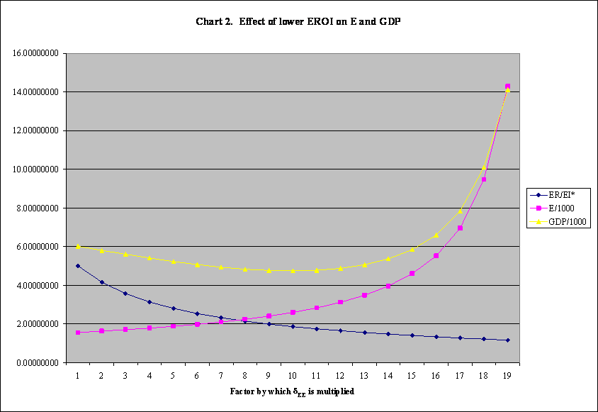
The stored results for Exercise 7 show that as the value of ER/EI decreases monotonically with increases in value of δ_EE, which is the constant by which the number of energy units delivered (ER - EI) is multiplied to determine the number of energy units required to produce it (EI) at each pass through the economy. As ER/EI approaches 1.0 from above, the total energy budget and total production approaches infinity. Thus, in a modern society the replacement of a high ER/EI primary energy technology by a low ER/EI technology will cause great economic suffering well before it become theoretically infeasible. This experiment was done properly in http://www.dematerialism.net/Mark-II-Economy-CSP.xls. The results are graphed in Chart 2, which appears in Experiment 9 below.

Experiment 8

Press <c>v. The energy (E), GDP, and E/GDP for that portion of the economy modeled in the dedicated ER/EI computational section is computed and stored in DV45::DX48. Store DV46:DX46 in DV47:DX47 to zero out DV48:DX48. Since there is only one commodity, namely, energy, it should not be surprising that an increase in EX (= ER - EI) of 1 EU would produce a change in the GDP that, when multiplied by (E/GDP)_o, gives a value of EI such that (EX + EI)/EI = ER/EI agrees with the ER/EI computed directly. Change the value of DV44 to 1.0 and read the estimated ER/EI in DV43. Compare it to the value of ER/EI in DO43, and don’t forget to change DV44 back to zero.

Experiment 9

A new spreadsheet that represents the Mark II Economy solves the problem of keeping the fractions of the population associated with each sector constant regardless of changes in political economy or changes in δ_EE, the number of energy units required to yield a net energy to the rest of the economy of 1 EU. One EU represents ER – EI^o, where EI^o is the lowest value of energy invested one might conceivably consider, namely, a value that considers direct energy costs only at the first level and pointedly excludes even the normal energy expenses of the employees of the energy sector. I agree that I am remiss in not discussing ER/EI^o = (1 + δ_EE)/δ_EEand tabulating it for each of the cases as this is the ratio that gives the highest value of ER/EI. In the new spreadsheet at http://www.dematerialism.net/Mark-II-Economy-CSP.xls, I have computed and tabulated the Payback-Time Factor as the payback time required to amortize all of the energy costs that would not have occurred if no energy had been produced divided by the payback time calculated from ER/EI^o, the most optimistic payback time. Also, the new spreadsheet has two charts so far. Chart 1 shows the reduction in energy and labor required to produce an invariant standard of living and the increase in ER/EI* as the political economy improves in discrete steps from the unsustainable market economy with two-tier salaries represented by the Base Case (BC) to the No-Managers Case (NM) to the No-Commerce Case with commissars (NC) to the No-Commerce-No-Managers Case (NCNM).

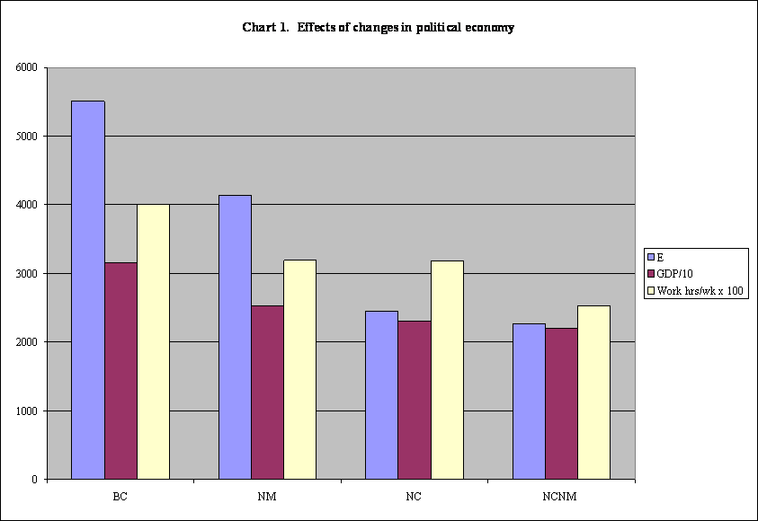
Chart 2 shows the rise toward infinity of the energy budget as ER/EI* diminishes toward 1.0; however, Chart 7 illustrates the phenomenon much better. Therefore, it will be shown next in place of Chart 2, and it will serve for all such experiments to avoid wasteful duplication. Look for other results between columns DC and DZ.

Experiment 10

In the earliest versions of the spreadsheet, the f_ijand the p_i were adjusted until the fractions of consumer expenditures, m_i, and the fractions of the energy budget, e_i, going to the various sectors resembled somewhat the US economy. With a converged solution in hand, it was advisable to fix the η_i and the δ_ij and let the prices, p_i, and the f_ij float as this arrangement corresponds best with physical reality. Indeed, at that time, the problem of matching m_i and e_i to the US economy by adjusting the f_ijand the p_iseemed insurmountable. However, in http://www.dematerialism.net/Mark-II-Economy-CSP.xls, with the simultaneous solution of cash balance equations to obtain the x_i and p_i, it is easy to match the e_i for the Mark II Economy to the e_i for the US economy by replacing δ_iE by (e_i^US/m_i^II)δ_iE, which is done by pressing <CS>Q, solving the cash balance equations, and repeating. With the e_i matched, η_i is replaced by (m_i^US/m_i^II)η_iwith <CS>U. A successful sequence of operations is <CS>Q followed by <CS>P once or twice (to solve the cash equations), and repeating until e_i match. When the e_i match, press <CS>U and <CS>P repeatedly until the m_i match. If the e_i are no longer matched, repeat entire sequence to convergence. Chart 3 replaces Chart 2 for the new Base Case, which resembles the US economy as closely as it is possible to do with a Mark II Economy; however, Chart 7 above is a better picture. I have not bothered to contrive a method for updating the deltas that does not obliterate the formulas in CF6:CF11; however, the macro executed by pressing <C>t will save the new values of CF6:CF11 in CC6:CC11 and repair the damage.

Experiment 11

In an effort to push the economy closer to infeasibility I decided to allow the fractions of the population dedicated to the manufacturing, transportation, and energy sector in http://www.dematerialism.net/Mark-II-Economy-CSP.xls to be altered by multiplying them by the values of z in CR3:CR5 and iterating until the production per capita in each of those sectors was what it had been with the original value of δ_EE. This could be done until the value of δ_EEreached seven times its original value at which point the population of the commercial sector would have become negative. Therefore, the populations were allowed to remain constant once again and the factor by which δ_EEwas multiplied was pushed all the way to 10.0. The value of ER/EI* indicated in CT380, which is a snapshot of the results, is 1.085; but, this cannot be correct because the negative number in CV362 indicates that EI* is infinite. Thus, at some value of δ_EE less than 10.0 times the original value of δ_EE, δ_EE has passed the point at which ER/EI* is arbitrarily close to 1.0, and ER/EI* is now undefined. The production of MUs, TUs, and EUs had become impossibly high. The economy would have broken down long before this occurred. In any case, I proved to myself that up to a fairly high value of δ_EE I can retain the original values for production per capita in the manufacturing, transportation, and energy sectors by altering the fractions of the population appropriately.

Experiment 12

So far, we have assumed that workers in the commercial sector earn no more than workers in the other sectors. Perhaps, in an American-style economy it might be more reasonable to assume that workers in the commercial sector are principally college graduates; therefore, in this experiment, we have increased their pay by 50% (CV28 = 1.5), which, perhaps, is still conservative. In any case, we wish to find out how much energy and how much labor would be saved by switching to a natural economy with economic equality and no commerce. We assume, as usual, that, in a society where corruption is impossible, the cost of economic planning is negligible. This is a reasonable assumption, but I should say why much earlier in this paper.

In any case, snapshots of the results can be found in the rectangle CP421::DA494 with 65.1% of the energy saved in CT490 and 80.5% of the labor saved in CT491. Indeed, the “elephant in the living room” is the high cost of commerce and the market.

Note. It is important in http://www.dematerialism.net/Mark-II-Economy-CSP.xls to restore the value in CV28 to 1.0 before trying to converge any of the “better” cases, that is, better than the Base Case.

Experiment 13

In this experiment, the exercise begun in Experiment 12 is carried out systematically. In http://www.dematerialism.net/Mark-II-Economy.xls, the value of κ = {1.0, 1.4, 1.4, 1.0) in the Base Case is raised to κ = {1.0, 10.9, 10.9, 1.4}, which amounts to a managerial class that spends 100 times the amount spent by workers on their residences and manufactured goods and five times the amount spent by workers on transportation to account for the super-rich and to account for expensive cars and air travel. In this case, the savings in energy effected by switching to a natural economy amounts to 93%. The complete results are plotted in Chart 4: The need for a Natural Economy grows as American-style Capitalism becomes more wasteful, Chart 1on the spreadsheet.

In http://www.dematerialism.net/Mark-II-Economy-CSP.xls, due to ease of convergence with Newton’s method it is easy to plot increasing values of the components of κ and the commercial premium mentioned in Experiment 12 until a commercial premium of 1.9 is reached after which the fraction that must be retained to pay salaries in the energy sector exceeds 1.0 and the computation destroys the spreadsheet. One then re-loads the last saved copy. I do not know how to avoid doing this, so I save after each step is completed. Also, I disable the automatic save feature. The complete results are shown in Chart 5, Chart 4 in the spreadsheet. Again, it is important to reset CV28 to 1.0 before trying to converge the No-Commerce-No-Managers Case.

Experiment 14

In earlier experiments with lowering ER/EI*, we did not plot the behavior of the GDP, which is affected by the Mark II economic rule that the price of energy remain constant at one X dollar per energy unit. In Chart 5 of in http://www.dematerialism.net/Mark-II-Economy-CSP.xls, we were able to increase the factor by which δ_EE is multiplied all the way to 11.0 and plot E/1000 and GDP/1000 – probably because we are using Newton’s method with analytic derivatives. Regrettably, Chart 5 below shows only the first half of the original version but with smaller step size; therefore, refer to Chart 7 above.

Experiment 15

In this experiment on http://www.dematerialism.net/Mark-II-Economy-CSP.xls, I reduced the value of δ_EEto half of its original value when the factor by which it is multiplied is 1.0. Thus, the ER/EIs can be lowered in smaller steps. Chart 7 above is the result.

Experiment 16

Rather than try to solve sixteen equations by Newton’s method, I decided to keep the entire population of each sector on active duty and reduce the hours worked per week to take advantage of the savings in overhead in the “better” cases as reflected in the Production ratio in DR50:DR53. The average value in DR54 is shown in CT31, although the production ratios for the sectors should be equal. This has proved more interesting than merely duplicating the results in Mark-II-Economy.xls with faster convergence. Please see http://www.dematerialism.net/Mark-II-Economy.xls. Click Enable Macros; then, when the message “This workbook is linked to other data sources” appears, click Don’t Update. Open up the macros menu on the tools drop-down menu to determine what keys to press to execute the macros or see Table 2 in Appendix A. For one Newton step, press <CS>O. If, in the No-Commerce-No-Managers Case, the production ratio is 0.666, the work day could be reduced from eight hours to five hours and twenty minutes.

Experiment 17

According to Figure 8E in http://tinyurl.com/ksk5z, in 2003 the top 10% earns 43% of the income in the United States. Therefore, to simulate American inequality in the Mark II Economy, the managers should earn 6.79 times what the workers earn. Since, in a steady-state economy, everyone spends everything he earns (sic), the expenditures on residential units and manufacturing units must be 1.96 times what they would have been if managers had been paid the same as workers. Also, by iterating on δ_EE, I have matched an average ER/EI^o of 20 for the slate of fossil fuels consumed in the United States.

As ER/EI^o is reduced to about 3.0 for the average renewable primary energy technology, we can determine the new energy budget. Assuming a current energy budget of about 100 quads, the energy requirements for ER/EI^o = 3.0 will be almost four times Maximum Renewables as determined by Pimentel. On the other hand, if we have shifted to a natural economy, the energy requirements will be less than 92% of Maximum Renewables with one-tenth the number of transportation units and one-half the number of residential and manufacturing units, which is possible since only about 42% of the work force is working and at about half-time too. Indeed, passenger cars and planes will find their proper places in museums, and the era of over-consumption will have ended.

That said, I continued to search the internet until I found a less egregious figure for the percentage of the income earned by the top 10%. According to Table 3.2 in http://tinyurl.com/r4wyr, after taxes and government subsidies, the top 10% earned 31% of the income. Therefore, to be conservative in my claims for the natural economy, I have used this number, which leads to an energy requirement for the steady-state market economy 3.86 times Maximum Renewables and an energy requirement for the natural economy 1.07 times Maximum Renewables computed as before. So, until the population begins to diminish after many of the incentives for excessive procreation are removed, the people will have to avail themselves of a small amount of non-renewable energy or conserve more energy. By reducing the amount of energy required to produce one agricultural unit by 50% (changing the number in CC12 to 0.5), the energy requirement for the natural economy is reduced to 88% of Maximum Renewables. If you do this for the No-Commerce-No-Managers Case, don’t forget to change it back to 1.0.

The latest version of http://www.dematerialism.net/Mark-II-Economy.xls has two new macros. Try the following:

1. Press <CS>D to set the variables for the natural economy (No-Commerce-No-Managers Case).

2. Press <C>v to change the factors that multiply δ_iE, i = A, R, M, T, E, C, to account for the huge savings in energy in a natural economy due to extraordinary conservation measures.

3. Press <CS>O repeatedly until the number in CV14 is less than 10^-11, which shows that the balance equations are well satisfied.

4. Press <CS>V to set E_o and GDP_o.

5. Paste the values in CT32:CT36 into CT191:CT195 using the Paste Special feature of MS Excel if they are not already equal to them.

6. Press <C>a to return to the Convergence Section and notice in CT33 that 75.0% of the base-case energy is saved by switching to a natural economy. The new energy budget is 96.5% of Maximum Renewables as shown in CV39.

7. Press <C>u to restore the base-case values for the factors that multiply δ_iE, i = A, R, M, T, E, C.

8. Press <CS>A to restore the base-case variables.

9. Press <CS>O repeatedly until the Base Case is converged.

10. Press <CS>V to set E_o and GDP_o.

11. Press <C>a to return the cursor to the Convergence Section and to re-format the spreadsheet.

Chart 9 below is a little dated, but it shows the general effects of changing political economy, e. g., substantial reductions of the energy budget.

Additional Experiments

I shall report on additional experiments as I go along.

Summary

Please see http://www.dematerialism.net/remarks.htm for an introduction to this section. In particular, “Remarks” provides an explanation of the Autonomous Alternative Energy District

In Experiment 4 in which one unit of each of the four commodities is invested one at a time, the change in energy determined by the spreadsheet, ΔE_calc, may be greater or less than the change in energy computed by multiplying one unit by the E/GDP ratio (ΔE_est), but it does not vary by as much as a factor of two in these experiments. See DS31:DS34. In Experiment 1 where 1 XD is distributed across the economy, the two quantities are precisely equal. See DO26, DO27, and DO30. This proves that the Energy Invested in ER/EI for the Autonomous Alternative Energy District may be computed by multiplying the monetary costs by the E/GDP ratio.

Very good agreement was found in Experiment 5 for a distribution over the RUs, MUs, and TUs (but not AUs) in the proportion they are distributed over the economy at large; and, in Experiment 6, order of magnitude agreement was found for a distribution over just manufacturing and transportation. Finally, the sum of the products of the calculated energy change over the estimated energy change for the investment of one unit of each commodity separately times the monetary fraction of that commodity’s contribution to total consumer spending is 1.0 exactly if the sum is taken over all four commodities. See DU30:DU35.

In Experiment 2, we demonstrated three important points concerning economic change from (A) an American-style market economy to (B) a Chinese-type communism with markets to (C) a Soviet-style communism with a privileged commissar class to (D) an egalitarian natural economy without markets. In Experiment 3, we tabulated emergy data in a Mark II Economy. Finally, in Experiment 7, we explored what happens if alternative energy technologies with progressively lower ER/EI*s are embraced by all of society.

Undoubtedly, I will continue adding to The Experiments subsequent to the release of this early draft on July 16, 2006. Hopefully, the people who see this will offer useful suggestions, corrections, valuable insights, and, perhaps, solutions to the problems I have left unsolved.

Future Work

What we need is a computer whiz who can turn the Mark II economy into a scintillating computer game complete with fancy graphical user interface, animation, etc. In short, make it fun and easy to use and understand.

I hope that a person or persons younger and more talented than the author will produce a simplified model economy that looks much more like a real economy with many more sectors than four and sub-sectors and banking and profit-taking and government and perpetual war etc. Then, we would have an idea what is required of a primary energy source, e. g., alcohol from switch grass or bio-diesel from algae in aquaculture, if the entire economy (including perpetual war and everything else useful or not) ran on that one primary energy source. We would be able to tell if the energy produced could power the entire economy. All the energy costs whether they contributed to producing energy or not must not exceed the energy produced by the energy technology under investigation.

Then, we could cut out a few of the frivolous expenses, then more frivolous expenses, and eventually get rid of parasitical businessmen and see if that results in a sustainable economy. When we were done with that stage of the experiment, we would have a good idea about what sort of economy is sustainable with that primary energy source and what sort is not. We might then repeat the same exercise with a second primary energy technology. Etc.

Finally, we would introduce multiple energy sources and solve the matching problem for a realistic economy. This would all be based on the kinds of experiments I did with the Mark II Economy. I nearly ruined my health with the Mark II Economy, and this is a simple economy. Clearly, I need help. Unfortunately, I can’t be certain that anyone will take the work seriously for all the reasons people find NOT to do the right thing.

If we do this experiment, we will see that it is impossible to produce enough sustainable energy to support monetary systems and markets. Also, in a sustainable eco-community, who wants to waste valuable time accounting for who spent what on what? The members of the community will be pretty busy with gardens and other things they need to live. The butcher, baker, and candlestick maker will be busy enough without collecting bills, keeping books, or maintaining a cash register. (How many times have you found what you wanted in a store in five minutes but took a half hour to pay for it? Only yesterday, I walked into Home Depot knowing that I wanted 10 sheets of plywood for hurricane shutters but spent nearly an hour paying.) Or, consider my separate medical files: one for actual medical considerations like referrals, prescription information, copies of physicians’ notes, etc. and a second for medical billing. The file for billing must outweigh the other file by a factor of ten at least.

Even if we don’t do the above experiment, my conclusion that the economy cannot afford markets and monetary systems has been validated by the numerical experiments in http://www.dematerialism.net/CwC.html that were summarized in http://www.dematerialism.net/demise.htm.

Final Thoughts

In the case of alcohol from biomass, the best methodology for determining ER/EI can matter very much to people who are directly involved, however it will probably not have any effect upon the rest of us unless this technology plays a substantial role in the energy economy of the United States. Moreover, for farmers, for example, who try to anticipate their motor fuel requirements by local action in the shadow of Peak Oil, conventional analysis will work fine, as they shall not incur business costs in connection with the local use of biomass technology.

However, suppose the same discussion were to be applied to nuclear power installations. In a capitalist economy, such as some people still believe will be part of America's future, nuclear would become the principal source of power to “keep the train rolling”. The conclusion would be a matter of life and death for a huge population. The effects would be felt locally whether one approves or disapproves of national policy.

Piecing together various types of alternative energies – unless nuclear energy be considered an alternative – cannot “keep the train rolling”. Personally, I favor the soft-energy, “Earth as a Garden”, natural economy, but this requires a political sea change that must sweep the entire nation. It cannot be managed locally. We can act locally, but we must communicate globally. If we do not effect political change nationally, global events will swamp local action, which will be viewed as nothing better than Personal Salvationism.

Rapidly introducing energy-saving and renewable-energy technologies will have enormous energy consequences that many of us will not like. Many people believe that the necessary technological changes cannot occur without the help of entrepreneurs, and they may be right. See, for example, http://groups.yahoo.com/group/globalvillages/message/501 for a rebuttal to some remarks made by me.

The ultimate goal is to prevent Die-Off. I am trying to convince the reader – not necessarily with ER/EI studies; but by showing that, if commercial activities are not included in the EI computations, society will be left with many activities that have no energy to support them. If this is not recognized a priori and the required political changes do not take place, commerce will continue to suck the blood out of the economy to the detriment of feeding the poor, for example. Commerce won't stop simply because no energy has been provided to carry on its activities. It will continue to misappropriate the energy needed for vital activities, since commerce has been and will continue to be a predatory economic parasite.

Traditionally, socially progressive thought has tried to effect change by appealing to our moral natures. Peak Oil presents us with a challenge and an opportunity. Perhaps, for the first time during my lifetime, it is possible to demonstrate mathematically the need for social change. (The single most powerful intellectual tool of which I am aware is a properly closed balance equation.) Perhaps, very few people are accessible through their mathematical propensities, but those who are can be stunningly convinced of a need to change their minds when confronted with mathematical proofs. I wish to take advantage of that. Unfortunately, I shall put a number of people to sleep who do not wish to be bothered by mathematics however elementary. (I know people who are bored by their children's grade school math homework.) I hope that people like you take the trouble to understand the mathematical argument presented here and make it evident to people who are bored by mathematics by making it interesting in some other way.

Houston, Texas

July 16, 2006

Revised August 4, 2006

Tables of Macros

These tables are obsolete except for a few important macros.

Table 1. Table of Macros for http://www.dematerialism.net/Mark-II-Economy.xls
BC	Initialize Base Case	<CS>A
NM	Initialize No-Managers Case	<CS>B
NC	Initialize No-Commerce Case	<CS>C
NCNM	Initialize No-Commerce-No-Managers Case	<CS>D
Iter A	Set formulas in DA3:DA5 for Base Case	<C>s
Iter B	Set formulas in DA3:DA5 for all other cases	<C>w
GDPE	Set GDP_o to GDP and E_o to E (to be executed immediately after current case is converged)	<CS>V
Computation	Sends cursor to computation section of spreadsheet and auto-fits	<C>d
EROEI	Sends cursor to EROEI section of spreadsheet and auto-fits spreadsheet	<C>b
Show	Sends cursor to convergence section of spreadsheet and auto-fits	<C>a
SeeDELS	Sends cursor to δ_ij section of spreadsheet and auto-fits	<C>f
Results	Sends cursor to results section of spreadsheet and auto-fits	<C>r
PowerM	Performs several iterations of convergence routine for Base Case	<C>m
PQX	Performs one iteration of the convergence routine for the Base Case	<CS>M
PowerZm	Performs several iterations of the convergence routine for better cases	<C>o
Ziter	Updates the fraction of the M, T, and E sectors on active duty	<CS>Z
ProdInit	Sets the initial production for each of the sectors to the current value	<C>p
Piter	Updates the prices	<CS>P
PI	Updates the fractions of the population associated with each sector	<CS>Q
Xiter	Updates the fraction of gross cash retained for salaries for each sector	<CS>X
Init
PIConst
PPI
RestartBC
RestartNMNCNCNM
ToResults	Sends cursor to results section of spreadsheet and auto-fits	<C>v
XP

Table 2. Table of Macros for http://www.dematerialism.net/Mark-II-Economy-CSP.xls
BC	Initialize Base Case	<CS>A
NM	Initialize No-Managers Case	<CS>B
NC	Initialize No-Commerce Case	<CS>C
NCNM	Initialize No-Commerce-No-Managers Case	<CS>D
StoreX	Stores variables in CQ6:CQ26 in CW3:CW26	<C>e
RestoresX	Pastes variables in CW6:CW26 into CQ3:CQ26 (used in finite difference derivatives)	<C>w
IncrX	From Sheet 3, pastes values from CZ6:CZ26 into CQ6:CQ26, and ends on Sheet3 with auto-fixed formats (used finite difference derivatives calcs)	<CS>I
GDPE	Set GDP_o to GDP and E_o to E (to be executed immediately after current case is converged)	<CS>V
Computation	Sends cursor to computation section of spreadsheet and auto-fits	<C>d
EROEI	Sends cursor to EROEI section of spreadsheet and auto-fits spreadsheet	<C>b
Show	Sends cursor to convergence section of spreadsheet and auto-fits	<C>a
SeeDELS	Sends cursor to δ_ij section of spreadsheet and auto-fits	<C>f
NR10	Takes one Newton step in Base Case	<CS>O
TenNR10s	Executes <CS>O ten times	<CS>P
NR16	Takes one Newton step for better cases	<CS>Z
TenNR16s	Executes <CS>Z ten times	<C>z
UpdateDEL	Updates δ_iE to match US energy use data	<CS>Q
UpdateETA	Updates η_i to match US consumer purchasing data	<CS>U
QUP	Executes <CS>Q, <CS>U, and <CS>P once	<CS>W
TenW	Executes <CS>W ten times	<C>w
FixDELs	Restores formulas for δ_iE and their stored values in CC6:CC11	<C>t
ProdPerCapInit	Sets the initial production per capita for each of the sectors to the current value	<C>q
ProdInit	Sets the initial production for each of the sectors to the current value	<C>p
GDPEInit	Sets Base-Case E and Base-Case GDP to the current values	<C>r
Low	Sends the cursor to the finite difference derivatives calculation on Sheet 3	<CS>Q

Appendix B. Table of Spreadsheet Values (deleted)

Appendix C. Convergence Mathematics

To be supplied later

Note. The charts that are obsolete have been deleted.

Table of Contents

What’s New (September 19, 2006)

To the Reader

The Experiments

Tables of Macros

Appendix B. Table of Spreadsheet Values (deleted)

Appendix C. Convergence Mathematics